Quick Start Guide

There are two ways to get started, and both end in the same place: a running StreamPipes with live data on a dashboard.

• Try it in a minute. One docker run starts the complete platform in a single container, with a demo plant already set up. Best for a first look, a demo or a workshop.
• Install it. Docker Compose starts the regular multi-container setup that you can keep and grow. Best when you want to connect your own machines.

Whichever you pick, the second half of this page walks you through building your own first flow: an adapter, a dataset, a chart and a dashboard. That part takes about ten minutes and needs no external machine or broker.

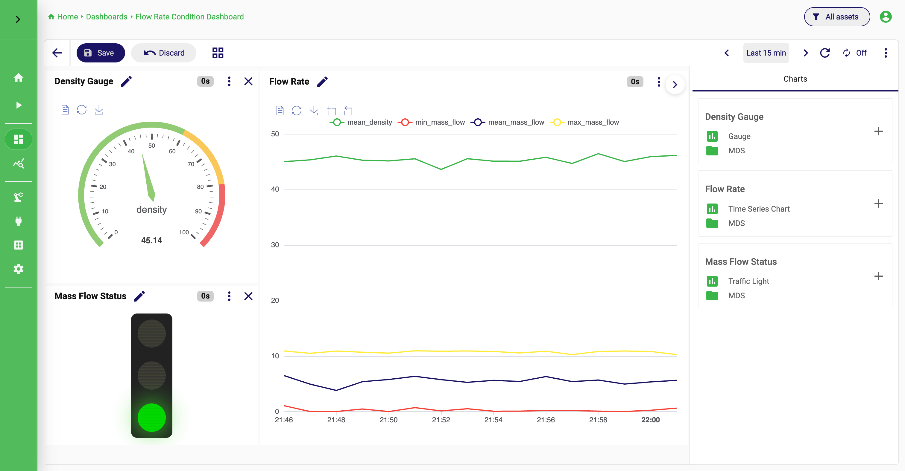
The result: a dashboard built from a chart on persisted data

Prerequisites

You need Docker on Linux, macOS or Windows. On macOS and Windows that means Docker Desktop, with at least 4 GB of memory assigned to it. The Compose installation also needs Docker Compose, which comes with Docker Desktop and with recent Docker Engine packages. Use a current Chrome, Firefox or Edge.

Install Docker

Go to docs.docker.com and follow the instructions for your operating system. Check the installation with docker run hello-world before you continue.

Option 1: Try it in a minute

The all-in-one image runs CouchDB, InfluxDB, NATS, the StreamPipes core, the IIoT extensions and the UI in one container. On first start it seeds a fictional company with simulated machines, so you see live data without connecting anything.

docker run --rm -p 80:80 apachestreampipes/all-in-one:dev

1. Open http://localhost. The services take about a minute to boot. The UI shows a progress screen and moves on by itself when the core is ready.
2. Sign in with admin@streampipes.apache.org and the password admin.
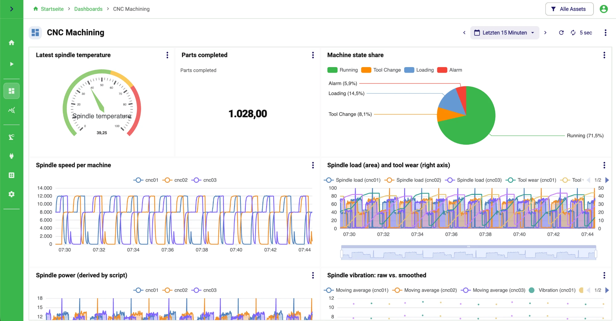
3. Explore. The demo comes with running adapters, pipelines, datasets, charts, dashboards and a modelled plant. A good first stop is Dashboards, for example CNC Machining below, then follow the links from the asset on the home page to the adapters and pipelines behind it.

One of the demo dashboards: KPI tiles, the machine state share and trends per machine

The dev tag follows the latest build of the development branch. From the next release on, latest and version tags such as 0.99.0 are published as well.

What to look at

The demo is a water works and an automotive supplier plant. Every machine is a simulated adapter that alternates between normal operation and an alarm phase every 30 seconds, which is what the analytics pipelines react to.

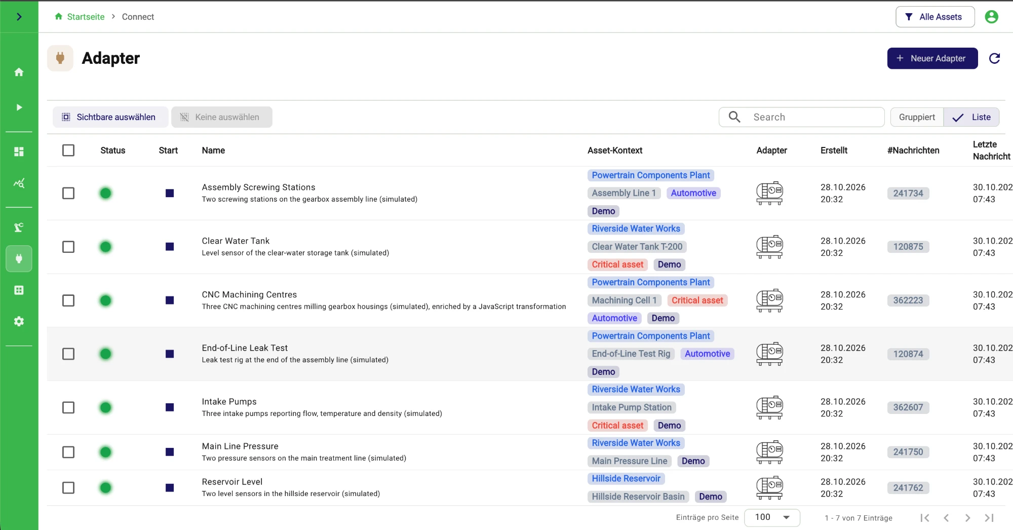
• Home shows the counters, the asset table and both sites on a map (toggle Map).
• Dashboards has an overview per site, detail dashboards per area, and Shop Floor Display, a dashboard in slide view for a screen on the floor.
• Charts contains about 40 charts across most chart types, from KPI tiles and gauges to histograms and heatmaps.
• Pipelines has the persist pipelines plus a few analytics pipelines: pump overheating detection, tool wear warnings, NOK joint detection, failed leak tests.
• Assets holds the plant structure with sites, areas, labels and links to everything above.
• Adapters lists the simulated machines. Open CNC Machining Centres to see a JavaScript transformation script that derives spindle power and a tool wear class before the events reach any pipeline.

The seven simulated machines, each linked to its plant, area and labels

Everything else works like a regular installation. You can add adapters, build pipelines and create charts. Stop the container with Ctrl+C. With --rm the data is discarded; drop --rm to keep the container and start it again later with docker start.

Good to know

Port 80 busy? Map another one with -p 8080:80 and open http://localhost:8080. Want an empty platform without the demo? Add -e SP_DEMO_SEED=false. Want a different admin password from the start? Add -e SP_INITIAL_ADMIN_PASSWORD=change-me. All options are described in the installer README.

The all-in-one image keeps its data inside the container and runs everything on one host. For anything you want to keep, use the Compose installation below.

Option 2: Install with Docker Compose

One command creates a folder, downloads the Compose file and its environment file for the latest release, and starts the default setup with NATS as the message broker:

mkdir -p streampipes-0.98.0 && cd streampipes-0.98.0
curl -fsSLO https://raw.githubusercontent.com/apache/streampipes/0.98.0/installer/compose/docker-compose.yml
curl -fsSLO https://raw.githubusercontent.com/apache/streampipes/0.98.0/installer/compose/.env
docker compose up -d

Then open http://localhost and sign in with admin@streampipes.apache.org and the password admin. The first start pulls the images and takes a few minutes; the login screen appears when the core is ready.

Login Screen

Before you use the instance for real, open the .env file and change the secrets and the admin credentials. The download page has the official source release and a variant of the command for the nightly build, and the deployment options cover Kubernetes, Kafka instead of NATS and extension services next to the machines.

If StreamPipes does not come up

The most common reason is an underpowered Docker setup. Check that Docker has at least 4 GB of memory, that all containers are running (docker compose ps) and read the logs of the backend container (docker compose logs backend). If the first start failed halfway, stop the stack with docker compose down, remove the volumes if you do not need the data, and start again.

Build your first flow

This part is the same for both options. You create one adapter with the built-in machine data simulator, persist its events into a dataset, create a chart on the dataset and place the chart on a dashboard. If you started the all-in-one image, the demo already contains adapters like this one; build your own anyway, it is the fastest way to understand how the parts fit together.

1

Connect a data source

Create one adapter in Connect so StreamPipes starts receiving events.

2

Persist the events

Enable persistence when you start the adapter, so the events become a dataset.

3

Check the dataset

Confirm that records arrive and the schema matches what you connected.

4

Create a chart

Query the dataset and show it as a time series.

5

Place the chart on a dashboard

Turn the chart into a view you can open any time.

Step 1: Connect a data source

1. Open Connect and click New adapter.
2. Choose Machine Data Simulator.
3. Pick the Flow Rate sensor and leave the wait time at 1000 ms, one event per second.
4. Click Next. The preview shows live sample events. No transformation script is needed, so click Next again.
5. In Configure schema, select the timestamp row and set its scope from Measurement to Timestamp.
6. Click Next to open the adapter settings.

Use Case

Why the simulator

The simulator removes protocol and network questions from the first run, so you can learn the StreamPipes flow itself. Connecting a real machine over OPC UA, MQTT or a PLC protocol works the same way; see the Connect guide when you get there.

If an adapter you expect is not in the list, install the extension first under Configuration > Extensions.

Step 2: Start the adapter and persist the events

1. Give the adapter a name, for example Flow rate test.
2. Enable Persist events. You can keep the suggested dataset name or enter your own.
3. Click Start adapter.

Persistence is the step that turns a live stream into data you can chart later. Without it you still have a stream for pipelines, but no history. Once the adapter runs, the live preview on its details page shows events arriving.

Step 3: Check the dataset

1. Open Datasets.
2. Find the dataset created by your adapter and look at its event count. It should grow by one per second.
3. Open the preview to see the records and the schema.

Dataset Overview

This is the checkpoint. If data reaches the dataset, the rest is straightforward. If the count stays at zero, go back to the adapter and check that it is running and that persistence was enabled.

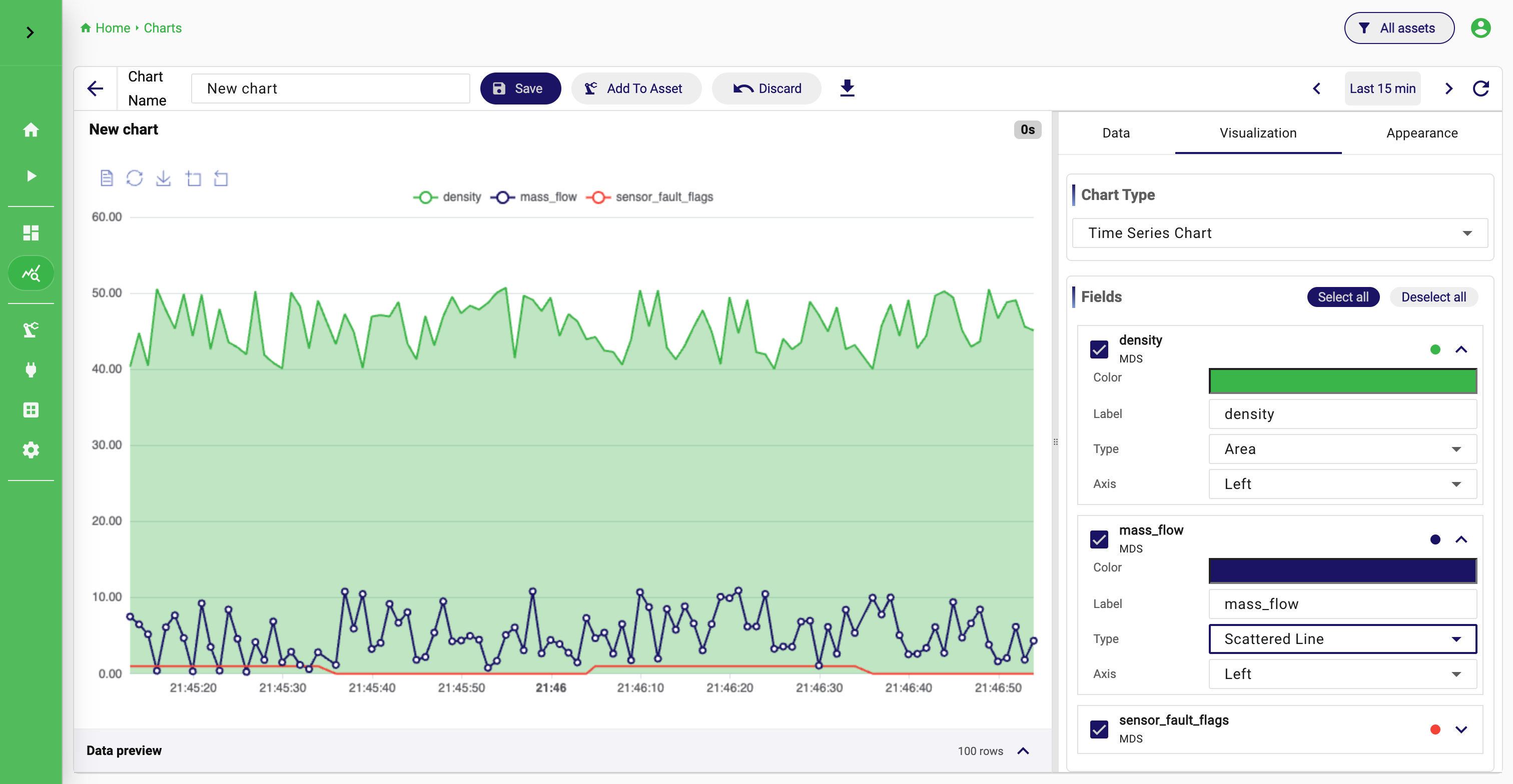
Step 4: Create a chart

1. Open Charts and create a new chart.
2. Select your dataset from the dropdown and keep Raw as the query type.
3. In the field selection choose Select all, then check the preview.
4. Switch to the Visualization tab and choose Time Series Chart.
5. Save the chart.

Step 5: Place the chart on a dashboard

1. Open Dashboards and create a new dashboard.
2. Open it and add the chart you just saved.
3. Arrange it on the grid and save the dashboard.

That is the complete first flow: a source, its history, a chart and a view. Everything else in StreamPipes builds on these four things.

Next: a pipeline

Pipelines work on the live stream before it is stored or shown: filter noise, calculate a KPI, detect a threshold, send a notification or write to an external system. Open Pipelines, start a new pipeline, drop your stream and a processor such as Numerical Filter on the canvas and end with a Dataset sink. The Pipelines guide explains the editor; the all-in-one demo has several finished pipelines to look at.

If something is missing

• The adapter or sink you want is not installed: add it under Configuration > Extensions.
• The dataset is empty: the adapter is not running, or Persist events was not enabled.
• The chart shows nothing: the dataset has no data for the selected time range yet, widen the range or wait a minute.
• The UI stays on the progress screen: Docker has too little memory, or the core is still starting. docker logs shows where it is.

Where to go next

• The use cases show complete scenarios such as condition monitoring, machine state tracking and alarm handling, with the adapters and processors they use.
• The feature guides for the parts you just used: Connect, Datasets, Charts, Dashboards and Pipelines.
• Assets organise everything by plant, line and machine; the all-in-one demo is a good example of a modelled plant.
• For the mental model behind it all, read Introduction, Terms and Architecture.